visustat_frame

With visustat_frame, continuous and discrete parameters can be mapped individually on color, shape and size for one timepoint.

Usage

visustat_frame(df, ...)

Arguments

df

dataframe of the form: df(track, time, X, Y, (Z,) mapping_parameters, ...)

image

character: filename of image

stack

logical: default: FALSE, single image file provided if time-resolved imagestack is used, set: TRUE

image.depth

numeric: set image bit-depth; just important if Z-projections are calculated

image.normalize

logical: normalize image

frame

integer: frame to be mapped

tracks

vector: defining tracks to be displayed

par.map

character: specifying parameter in df to be visualized by color

par.shape

character: specifying parameter in df to be mapped on shape

par.display

display option for mapping; default: TRUE, mapping is disable with: FALSE

par.max

numeric: defining upper range of color mapping

par.min

numeric: defining lower range of color mapping

par.unit

character: unit of the numeric mapped parameter

crop

logical: option for cropping images; default: FALSE

sub.img

logical: option for creating sub-images from specified tracks or pre-filtered df; default: FALSE

sub.window

numeric: size of the sub-images in pixels

sub.col

numeric: number of columns in which sub-images are arranged

tracks.size

numeric: size of tracks

tracks.alpha

numeric: transparency of tracks

tracks.length

numeric: length of tracks (in frames)

tracks.label

logical: when sub.img is used, display or hide track label

tracks.label.x

numeric: when sub.img is used, set x-position of label

tracks.label.y

numeric: when sub.img is used, set y-position of label

points.size

numeric: size of points

points.alpha

numeric: transparency of points

points.stat

character: display statistic; default: 'echo', for blurring; without blurring 'identity'

points.shape

numeric: set shape from ggplot2 shape palette

axis.tick

numeric: axis ticks in px

axis.display

logical: display axis

axis.labs

logical: display labs

unit

character: setting name of unit; default: 'px'

scaling

numeric: scaling factor for unit; default: 1

dimensions

numeric: specify whether the images are 2D or 3D. If 3D is selected the data is assumed to be in the form: df(track, time, X, Y, Z, mapping paramters, ...)

manual.z

numerice: specify Z-plane to be visualized if no projection or sub windows are used

scale.bar

logical: show scalebar; default: FALSE

scale.width

numeric: width of scalebar; default: 40

scale.height

numeric: height of scalebar; default: 10

scale.x

numeric: distance from left border of the image towards scalebar

scale.y

numeric: distance from bottom border of the image towards scalebar

scale.color

character: specify color from R-color palette or hexcode

interactive

logical: return the plot as an interactive plotly object. Not supported when using sub.img or crop modes.

Value

returns a ggplot2 plot-object which can be further modified

Examples

# import hiv motility tracking data
data('hiv_motility')
# get image files
images <- hiv_motility_images()
# run visustat_frame with default settings
visustat_frame(hiv_motility, image=images[15], frame=15, image.normalize=1)
#> par.map not specified
#> defaulted to: speed 
#> assuming: df(track, time, X, Y, mapping_parameters, ...)

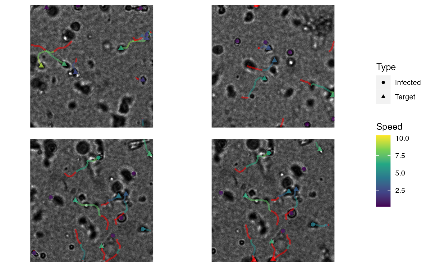
# run visustat_frame with specified settings
visustat_frame(hiv_motility,
   image = images[15],
   frame = 15,
   tracks = c(48, 66, 102, 108),
   sub.img = TRUE,
   sub.col = 2,
   sub.window= 300,
   par.map ='speed',
   par.shape ='type',
   points.size=2,
   image.normalize=1
 )

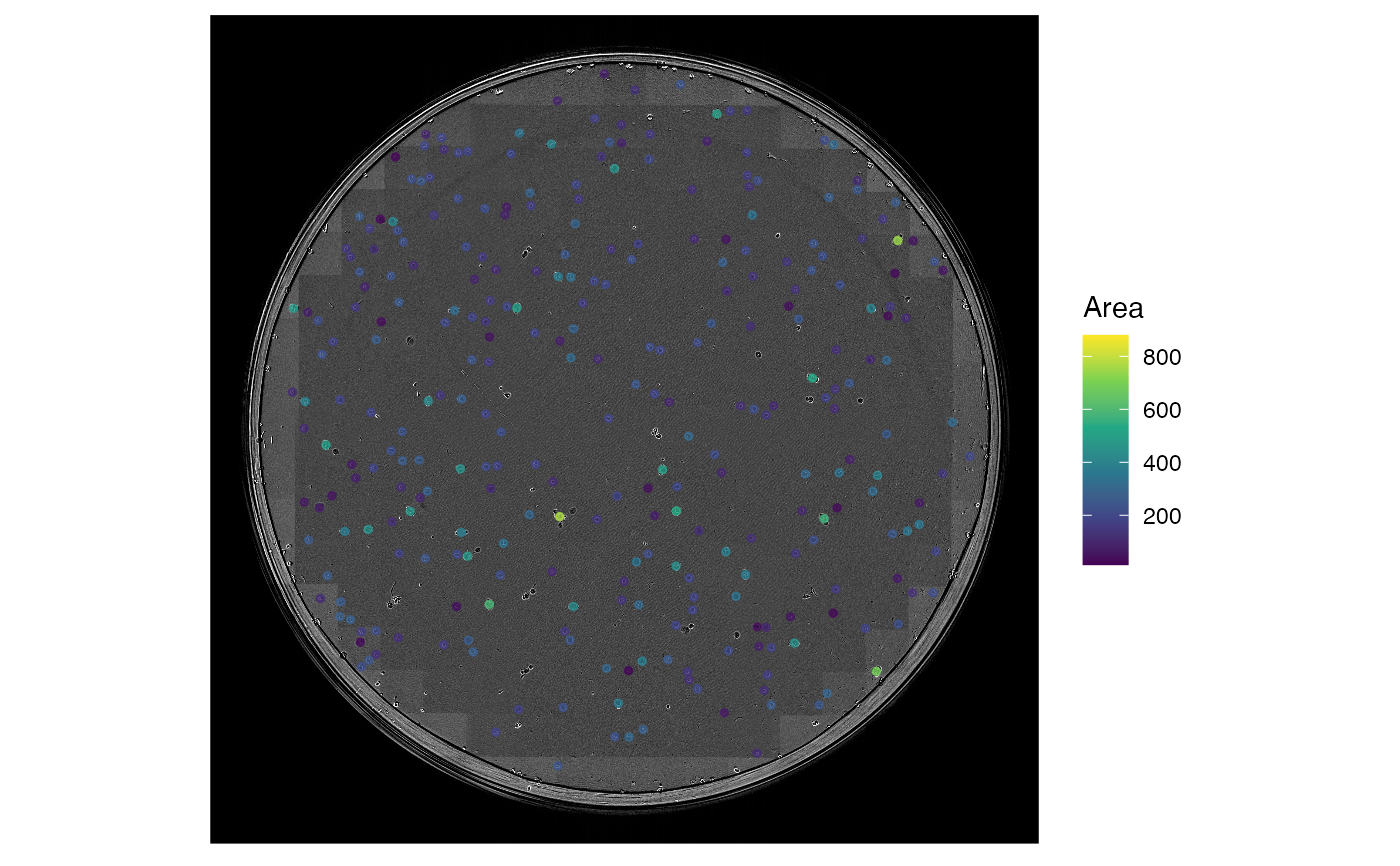
# import clonogenic assay colony growth data
data('clonogenic_assay')
# get image files
images <- clonogenic_assay_images()
# run visustat_frame with default settings
visustat_frame(clonogenic_assay, image=images[15], frame=15, tracks.length=0, axis.display=0)
#> par.map not specified
#> defaulted to: Area 
#> assuming: df(track, time, X, Y, mapping_parameters, ...)


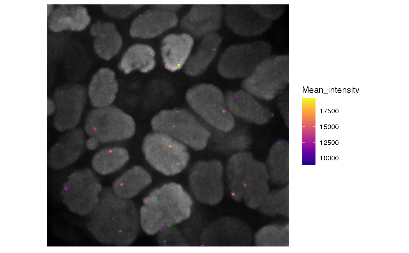
# import subcellular particle data
data('subcellular_particle_dynamics')
# get image files
images <- subcellular_particle_dynamics_images()
visustat_frame(subcellular_particle_dynamics,
 image=images[2], frame=2,
 tracks.length=0,
 axis.display=0,
 par.map='MEAN_INTENSITY') + scale_color_viridis_c(option='plasma')
#> Scale for 'colour' is already present. Adding another scale for 'colour',
#> which will replace the existing scale.